History
Introduction
Whether it is in the wake of a boat, a plane or even a cigarette, in the oceanic or atmospheric currents displayed in weather forecasts, in the frightening mushroom clouds and tsunamis, whether it hides in the disturbances created by a speeding car or a golf ball, turbulence’s complexity and beauty have inspired scientists, inventors, engineers and even artists, as they raised questions for thousands of years.
But what are its main features? How was such a complex phenomenon unraveled? What are the consequences of the developed theories on nowadays technologies?
Throughout this blog, several aspects of turbulence are explored, however, the general aim of the sections here below is twofold.
First, an historical description of turbulence’s understanding is provided.
This journey begins with a general description of the phenomenon, detailing its characteristics, early observations and interpretations. This section features some of the greatest minds of the last millennium, such as da Vinci, and explores the wonders and questions related to these tiny curls that are intrinsic to these complex flows.
Further on, a description of the main turbulent theories that emerged throughout the years is provided. The observers and scientists that influenced turbulent research are presented alongside with their ideas and theories.
The complexity associated to their theories and equations lead many to believe that a complete and accurate description of the phenomena they were trying to describe could never be obtained.
This complexity was successively tackled by the emergence of computers in scientific institutions, and soon enough, in houses. Therefore, the latest results and discoveries rose with the last century’s technological improvements, which are described in the third section of this blog. The discussion however remains open, looking towards the future and what it might bring to informatics, and successively, to sciences.
Alike any other scientific field, fluid mechanics and its discoveries always influenced scientists and engineers by providing new ideas for creating or improving already existing designs and technologies.
The second objective of this blog is therefore to depict turbulence through its impacts on innovation and engineering.
From the improvements in cars, planes, boats and even space shuttles, to the gigantic dynamics linked to weather forecast, even looking at the tiniest micrometric scales, this blog provides a description of the technologies that emerged in time, alongside with the discoveries presented in the first part.
Whether turbulence is sought or avoided, how can it be increased or reduced? How to identify a turbulent flow? The control and quantification of turbulence are indeed tedious and complicated tasks and a first section is entirely dedicated to these important questions.
The second section is dedicated to contexts where turbulence reduces the efficiency and performance of devices. Particular attention is paid to the case of drag reduction in the aerodynamics of planes and distribution networks such as pipelines, retracing some of the innovations that emerged from turbulence theories.
Afterwards, the last section discusses the uses and roles of turbulence in mixing, pollutants dispersion and energy harvesting through wind turbines. Here, the focus is on the possible uses of turbulence in technology and the different methods that can be implemented to benefit from it.
This blog provides a polished and accessible depiction to the rough and complex world of turbulent flows, guiding the reader in the natural historical flow, while regrouping the general ideas around recurring themes and concepts that inspired many, and shall hopefully inspire more.
Turbulence in the type vortex from an airplane wing [85]
History

The discoveries of Da Vinci
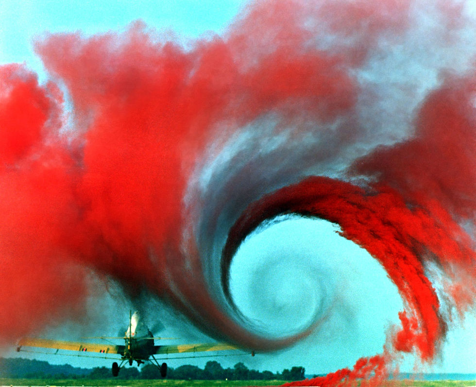
Turbulence, besides the complex equations and elaborate computer simulations techniques used to study it, is a very picturesque phenomenon. The eddying whirlwind patterns that we can observe in nature inspired many artists throughout the years.
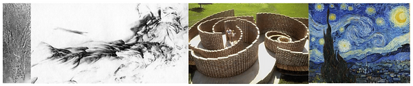
Figure I.1-1: "River Taw 22th January 1998" by Susan Derges, "The River's own hand" by Goh Shigetomi, "Marianthe" by Athena Tacha and "Starry Night" by Vincent Van Gogh [1]
Aside from the beauty of turbulent flows, it is their inherent complexity and ubiquitous presence that interests particularly physicists, mathematicians and engineers [2].
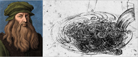
Figure I.1-2: Drawing of Leonardo Da Vinci about turbulent flows [3].
Leonardo Da Vinci, a leading artist and intellectual of the Italian Renaissance who brought the intuitions and schemes of inventions that inspired our current airplanes, helicopters, submarines and automobiles [4], provided a phenomenological description of the whirls he observed in agitated flows in 1507, and name it "la turbolenza" [3]. This is the first reported study of turbulence, supported by accurate drawings (Figure I.1-2).
"Where is turbulence in the weather generated? Where does the turbulence in the water persist for long time? Where does the turbulence in the water come to rest [2]?"
Even if the findings of Da Vinci found their origins 5 centuries ago, two aspects of turbulence are still considered today [3]:
The separation of the flow into a mean and a fluctuating part
The identification of eddies as intrinsic elements
Eddies are still considered to be the main structures responsible for and involved in turbulence [3].
Since the findings of Da Vinci, growing number of debates took place within the scientific community. Is turbulence a continuous or a discrete phenomenon? Is it deterministic or stochastic? The response to those questions changed in time and those "passing fads" found answers through history.
Should turbulence be modelled as a continuous or a discrete phenomenon?
The very phenomenon of turbulence is characterized by discrete structures in a continuous flow. As a fluid mechanics phenomenon, it is a continuous phenomenon as it is governed by the Navier-Stokes equations which are the foundation of fluid mechanics. But to what extent do the discrete structures depend on the continuity of the description?
With the arrival of computer science, it became a necessity to discretize the phenomenon in order to be able to simulate it as a computer can only manipulate discrete quantities. Conducting such a simulation procedure involves working on a set of equations which requires higher and higher momentums and thus are potentially infinite [3]. Considering that the more tasks the computer has to run, the more it impacts the performance in time, one need to close this set of equations in order to estimate a finite number of parameters which give the best simulation output possible.
Should turbulence be modelled as a deterministic or a stochastic phenomenon?
As a solution of Navier-Stokes equations, turbulence is a deterministic phenomenon: it is turbulence fully predictable given the initial conditions.But the phenomenon has many traits of a random phenomenon ruled by probabilities.
Navier-Stokes equations emphasize the deterministic side, showing that when the initial flow and boundary conditions are specified, the evolution is completely determined. Note that the presence of a non-linear term related to the velocity of the fluid makes it prompt to become turbulent when it is slightly modified. The deterministic chaos introduced by Lorentz also provided meaningful insights on the problem, namely that the system is sensitive to the initial conditions (i.e. even the slightest change in these conditions can cause the solutions to be very different).
The second point of view of this phenomenon, the stochastic one, has been described by Markov chains (and processes) [7] and Lagrangian stochastic modeling [8].
When large eddies become smaller
Richardson was an influential researcher in fluid dynamics of the early 20th century. He was also a meteorologist who performed the first numerical simulation for predicting weather [3].
He stated in 1922:
‘Big whirls have little whirls
that feed on their velocity,
And little whirls have lesser whirls
and so on to viscosity’
(Lewis F. Richardson, 1922) [5]
This statement connects the different scales of turbulence through to extremes, an injection scale and a dissipative one, as represented on Figure I.1-3.
Moreover, he suggested in 1926 a pictorial description of turbulence that he coined turbulent cascade.
Figure I.1-3: The Richardson's cascade
Fluid Mechanics
The progress in the study of turbulence was done step by step, requiring the understanding of fluid mechanics. Newton was the first to investigate the difficult subject of the motion of waves. He wrote the laws of motion and viscosity, introducing the idea of Newtonian fluid. This fluid has a viscous stress linearly proportional to its strain rate. The real fluids do not fit perfectly with this definition. Moreover it can be applied in some liquids and gases to simplify the calculations
After Newton, Bernoulli published the book Hydrodynamica where the fluid mechanics is organized around the conservation of energy. He states that when a fluid is in motion, if its velocity increases, then the pressure decreases.
In parallel with Bernoulli, d’Alembert applied the principles of the dynamics in bodies to the motion of fluids. He noticed that an incompressible fluid preserves its volume when moving from one place to another. When the fluid is elastic it dilates itself according to a given law.
At the same time, Euler developed the differential and the integral form of the equations of motion based on the principles of Bernoulli and d’Alembert. Their equations became known as Bernoulli equations.
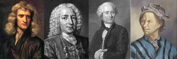
Figure I.1-4: The precursors of fluid mechanics [6].
In the middle of nineteenth century, Navier (looking at the molecular level) and Stokes (looking at the continuous point of view) created the Navier-Stokes equations (equation I.1-1).
Equation I.1-1: Navier stokes equations: the red represents the nonlinear term due the fluid velocity; the blue is the turbulence where ν is the kinematic viscosity; P is the kinematic pressure.
The equations describe mathematically the behaviour of flows and achieve the connection between the experimental and theoretical thoughts. Its formulation imply that turbulence is modelled as a continuum phenomenon. It shows that when the initial flow and boundary conditions are specified, the flow evolution is completely determined. Although, the presence of a nonlinear term related to the velocity of the fluid makes it prompt to become turbulent. The presence of this nonlinear term brought a mathematical obstacle to solve the turbulence problem within the deterministic framework. Consequently, this had led to many attempts to find the closure for the problem and instantiated the use of stochastic methods in the study of turbulence.

Figure I.1-5: Navier at left, Stokes (1819-1903) [6]
As it has been discussed, on the one hand-side, the turbulence phenomenon can be approached with continuous equations, although it is often more useful to discretize the phenomenon in order to implement computational simulations. On the other hand-side, there seems to be quite a controversy on whether turbulence should be seen as a stochastic or as a deterministic phenomenon, an issue that appears to be the order of the day. Consequently, many different theories on the turbulent flow have been developed throughout the years, leading to a diverse and fascinating history on this topic.
Illustration of the motion of water by Leonardo Da Vinci [86]

Modelling Turbulence
Scientists and, more generally, humans, have always found great inspiration and interest in nature and their surroundings. Many technological advances that were born from natural phenomena have been observed, studied, understood and finally replicated.
However, turbulent phenomena are still under debate because of their complexity and the multiple approaches under which they can be investigated. As a result, many theories regarding turbulence, as well as its causes and consequences were explored throughout the years.
As in many other scientific contexts, history played a major role in turbulence’s understanding and modeling. In this section, the main theories and hypothesis made by the scientific community to model turbulence and its complex features are highlighted.
A first interpretation of turbulence: Reynolds experiments
At the end of the nineteenth century, industry’s demand for scientific knowledge in turbulence led to the development of several new concepts. A theory that had a big impact on the comprehension of turbulence, emerged from Reynolds’s theoretical and experimental research.
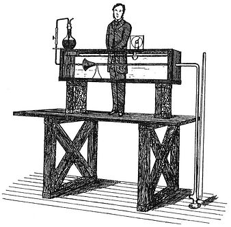
Figure I.2-1: Schematic representation of Reynolds running his pipe experiments [77].
With his pipe experiments, he gave a visual demonstration of a flow’s transition from a laminar to a turbulent regime (see Figure I.2-1). He defined a dimensionless quantity that is still nowadays used to quantify turbulence: Reynolds number Re, which is a ratio between the inertial and viscous forces. Its formula is given by Equation I.2-1., where L is the flow’s characteristic length, U its characteristic velocity and ν is the fluid’s kinetic viscosity. As shown in Figure I.2-2, turbulence occurs for high Re values.
Equation I.2-1: Reynolds number formula, where L is the flow’s characteristic length, U its characteristic velocity and ν the fluid’s kinetic viscosity.
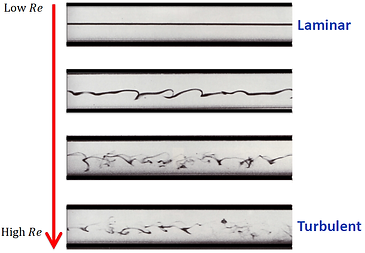
Figure I.2-2: Reynolds experiments, increasing reassociated to a regime evolution (modified from [96]).
Observing turbulent flows and extracting their main features, Reynolds had the idea to decompose the velocity field into a mean flow and a fluctuation, as graphically represented on Figure I.2-3.
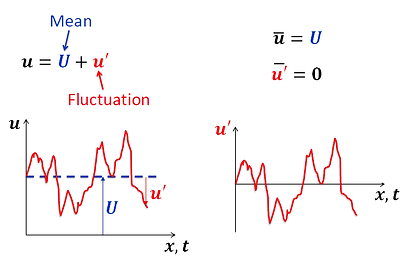
Figure I.2-3: Velocity field decomposition: mean flow and fluctuation (modified from [14]).
In order to quantify these newly introduced quantities, Reynolds considered time averages of the fluctuation. With this, he interpreted turbulence as an ordered and reproducible phenomenon instead of a chaotic and irregular one. This modelling of turbulence allowed him to eliminate the very complex interacting eddies Da Vinci first observed, focusing only on the mean flow (see Figure I.2-4).

Figure I.2-4: Averaging of a turbulent flow (modified from [95]).
Reynolds then showed that apparent stresses arise from the correlations existing between the different components of the fluctuating velocity. These apparent constraints are named Reynolds shear stresses. Combining his experiments with Navier-Stokes equations, he introduced the Reynolds averaged Navier-Stokes equations, given by Equation I.2-2, where the term in red represents Reynolds shear stresses. It is a non-linear term related to the flow’s kinetic energy. This term hides and represents a real challenge in the study of turbulence. Its interpretations and approximations led to the development of different models able to solve turbulent flows. The study revolving around this term is often named the turbulent closure problem.
Through their time-averaging, Reynolds developments laid the first stone of the main branch of the modern turbulence theory and later on initiated the stochastic movement in the studies of turbulence.
Equation I.2-2: Reynolds averaged Navier-Stokes Equations (RANS).
Prandtl’s boundary layer: an early attempt to aircraft modelling?
After Reynolds, Ludwig Prandtl came up with the concept of boundary layer [20], which is a combination of modelling and dimensional analysis. Considering a flow near a solid object, Prandtl was more interested in its behaviour at the surface of the solid boundary, where sharp changes of velocity can be measured, than its general bulk behaviour.
When a fluid flows over a solid surface, it is divided into two regions. The first one is the region external to the boundary layer, where the flow is determined by the displacement of streamlines around the body. In this region the flow is inviscid, and the pressure field is developed. The second region is the boundary layer, where, because of its viscosity, the fluid sticks to the contact point between the body and the fluid. At this point, the flow cannot slip away from the solid surface and has a zero velocity. However, inside this region, the fluid’s velocity increases rapidly from the contact point until the outer edge of the boundary layer (See Figure I.2-5).
The boundary layer has different shapes in laminar and turbulent regimes as in Figure I.2-6.
At first, the flow develops a laminar boundary layer. After a certain distance, the flow develops chaotic oscillations and begins its transition from laminar to turbulent. The exact location of that transition depends on the surface and occurs over a specific Re. In a turbulent regime the boundary layer thickens more rapidly than in laminar conditions because of the higher shear stresses at the body’s surface. The external flow interactions occur from the contact point with the body surface to the outer edge. Therefore, the mass, momentum and energy exchanges occur on a much bigger spatial dimension compared to laminar conditions.
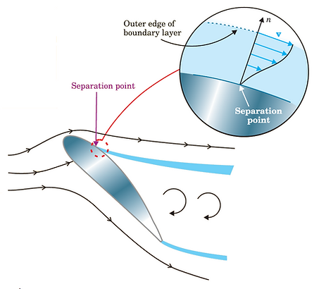
Figure I.2-5: Schematic representation of a boundary layer over a solid surface [27].

Figure I.2-6: Boundary layer, regime transition [78].
Another interesting phenomenon associated to flow over a surface is separation in turbulent conditions: The boundary layer can separate from the body entirely due to external conditions. In these cases, the boundary layer has low resistance against changes in pressure and it separates from the body surface and displays a different shape. Figure I.2-7 shows the different boundary layer separation phases.
With Prandtl’s modelling theories, it is possible to reduce Navier-Stokes equations into a simple form, local to the boundary layer. The resulting set of equations was very useful in practical problems where a rigid body is exposed to a turbulent flow. This set of equations naturally provided results and insights that influenced aeronautics and drag reduction.
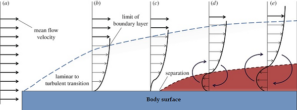
Figure I.2-7: Schematic representation of boundary layer separation [79].
Are turbulent structures deterministic and repeatable?
Even if Reynolds’s theory provided a fair amount of coherent results, the many whirls and eddies observed in turbulent flows still were a source of concerns and questions. How do they affect the mean flow? What are their characteristics? Are they really the result of a completely randomized motion?
From 1940 to 1975, experimental validation techniques had great influence on the formerly prevailing ideas [16]. Among these, an important observation made by Kline and Runstadler paved away a new trend in the very core of turbulence’s understanding [17].
Their ground-breaking discoveries identified a structured behavior to the previously considered chaotic flows and, for the first time, a certain quantifiable order is identified through experimental observation. This observation encouraged scientists not to consider turbulence to be the result of randomness, but to turn their interest to the phase behavior and the mean periods that could be identified in the observed flows, expanding Reynolds’s understanding of a turbulent regime.
Riding that new wave of thought, workgroups produced a fair amount of visual observations of structured turbulent behaviors. Among them, Brown & Roshko’s shadowgraph of a mixing layer produced by helium (see Figure I.2-8) identified two-dimensional vortices that keep their structure, even in a later growth stage.

Figure I.2-8: Shadow Photograph of a helium-nitrogen mixing layer ( A. Roshko, California Institute of Technology [18])
Dr. John Laufer [16] witnessed a radical change in scientists’ minds; Turbulence was considered to be described exclusively in statistical terms, meaning that its dynamics were considered to be unpredictable. However, these new experimental results showed that over well-defined periods of time, predictions and repeatability can also be observed, and turbulent flows exhibit characteristic shapes and sizes, as well as deterministic features.
In [19], a series of photographs of a mixing layer gives a visual description of the structures interactions encountered during turbulence (See Figure I.2-9). This exchange between a fast and slow streams results in the creation of an initially thin mixing layer, which further expands and develops into vortices that interact and undergo coalescence with very complex, but repeatable dynamics. These observations led the scientific community to further investigate the large and small scales observed in a turbulent flow, as their interaction certainly was the key to the understanding of this complex regime.
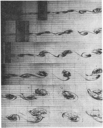
Figure I.2-9: Series of photographs of dye injected vortex coalescence (Winant &Browand Cambridge University Press [19]).
Turbulence: a multi-scale phenomenon
In the seventies, workgroups interested in turbulence already sensed that the large structures and their motion governed the later phases of the observed flows.
At the time [16] was published, speculations that these structures may have an influence in the early creation of the turbulent flows were being discussed.
Indeed, large and small scale structures displayed a distinguishable interaction in the unpublished experiments that scientists shared among each other. An emerging hypothesis -that nowadays is a key element in the largest and most complex fluid dynamics simulations- allowing to explain these phenomena can be described as follows:
Large structures dissipate energy through shear stresses until their sizes cannot sustain the additional stresses induced by their movement. That is to say, large structures, feeding on the mean flow energy, break down into smaller energy dissipating structures, up to the point where small vortices are reached, which will then dissipate energy through viscosity. This theory is nowadays often times referred as the turbulent energy cascade.
As it was previously mentioned, Lewis F. Richardson, a precursor to this theory, already hinted the existence of that cascade. His statements are surprising not only because of their accuracy, but also because of their earliness. This groundbreaking intuition would later on lead to Kolmogorov’s understanding of the multi-scale nature of turbulence.
Moreover, Richardson, who was a precursor in weather forecasting, realized that the fluid mechanics equations he was dealing with were almost too accurate to be solved, and would require three main ingredients [33]:
-
Effective equations.
-
Fast numerical algorithms.
-
A large number of simultaneous human computers.
One of his quotes almost predicts turbulence’s need for informatics and parallel computing:
“Imagine a large hall like a theatre ... A myriad computers are at work upon the weather of the part of the map where each sits, but each computer attends only to one equation or part of an equation. The work of each region is coordinated by an official of higher rank”
(Lewis F. Richardson, 1922) [5]
These early intuitions combined with the experimental observations made it clear that the understanding of turbulent phenomena would, in the future, have to take this multi-scale hypothesis into account. Dr. John Laufer concludes by saying that general averaging of the flow dynamics equations would only lead to “an unproductive closure problem”. The author also hopes that the split of the turbulence problem into a lower mode made of large structures, a lower scale random motion and their interaction, as suggested by experiments, can improve the theoretical formulations and elucidate a still very mysterious behavior: turbulence.
Eddies interaction: A complex and heavy problem
Historically, many scientists and observers had hinted the large and small scale interactions described by Richardson. However, a quantification of these complex phenomena was still missing.
In [9], the author considers the complexity related to turbulence to be a consequence of the fluid. The randomness associated to turbulence is much more complex, because it is not the motion of a few particles but rather of a volume of fluid which has continuously infinite degrees of freedom and the viscosity that makes it an energetically open system. The importance of Viscosity was highlighted by Taylor. In 1935, he hypothesized that for fully developed turbulence, the spatial average and the time average are equivalent and the dissipation rate depends on the viscosity and velocity gradients (shear) in the turbulent eddies.
In 1941, two papers published by Kolmogorov, [10] and [11], are generally considered as the origin of modern turbulence theory, because they introduce the concepts of scale similarity and universal inertial cascade. According to these papers, Kolmogorov introduced a definition for locally isotropic turbulence based on the independence of the distribution law from initial time, which is narrower than Taylor definition, but wider in the sense that restrictions are imposed only on the distribution laws of differences of velocities and not on the velocities themselves. Also according to the two definitions in [10], turbulence is considered to be locally homogeneous and isotropic in the domain G of the four-dimensional space.
According to the previously detailed Reynolds experiments, the transition from the laminar flow to turbulence requires an extra pressure difference between the entrance and the outlet of the pipe. This extra-pressure difference generates the kinetic energy of turbulence and compensates for the energy dissipation, so that in a turbulent steady state, the pressure per unit time is balanced by the energy dissipation rate of the turbulence.
In the view of Kolmogorov, turbulent motions involve a wide range of scales, from a large scale L at which kinetic energy of turbulence is produced by mean shear, to a micro-scale ƞ at which energy is dissipated by viscosity. In fact, the large scales are transferred through intermediate scales to the smallest scale ƞ, called Kolmogorov scale, where viscosity is strong enough to dissipate energy.
According to [14], the rate of energy transfer Π at large scales and the rate of energy dissipation ɛ at small scales are given by Equation I.2-3.
Equation I.2-3: Energy flux function and Dissipation rate[97].
At equilibrium, the energy flux function must be equal to the dissipation rate, as stated in Equation I.2-4.
This relation provides us with a ratio between the large and small scales, given by Equation I.2-5.
Equation I.2-5: Kolmogorov’s scales ratio [97].
From a deterministic or statistical point of view, the transition process appears to be so complex that it is difficult to expect any physical law to describe these phenomena. According to [9], the secret of the success in the theoretical study of turbulence exists in the idea of reductionism according to Kolmogorov's hypothesis. That is, to separate small-scale components of turbulence from the large-scale variety of turbulent flows and to look for the physical laws governing the small-scale component. Kolmogorov considered that although large-scale structures of turbulent flows may be different from each other, a local equilibrium state exists for small eddies, which is universal to all turbulent flows. Then, he suggested that this local equilibrium state is stationary, isotropic and governed by external parameters which represent the energy inflow and outflow to and from these small eddies. This proposition is called Kolmogorov's local equilibrium hypothesis.
The local equilibrium hypothesis is important, because it provides the basis for the Kolmogorov’s similarity hypotheses, which, according to [10] and [15], are stated as follows:
-
Kolmogorov’s first similarity hypothesis: At sufficiently high Reynolds number, all small-scale statistical properties are uniquely and universally determined by the mean dissipation rate ε and the viscosity ν.
-
Kolmogorov’s second similarity hypothesis: In the limit of infinite Reynolds number, all small-scale statistical properties are uniquely and universally determined by the mean dissipation rate ε and do not depend on v.
These hypotheses were widely accepted at the time. However, in 1962, Kolmogorov, inspired by Landau and Oboukhov, refined his original theory to take into account the spatial fluctuations in the turbulent energy dissipation rate ɛ at scale ℓ. Indeed, Landau noticed that these hypotheses did not take into account a particular circumstance, which arises directly from the assumption of the random character of the mechanism of energy transfer from the large to small vortices. If the ratio between L and ƞ increases, the variation of the dissipation of energy should increase without limit, instead of having an asymptotic behaviour [12].
On the other hand, the study of Goto et al. [13] qualitatively investigate the validity of Kolmogorov’s local equilibrium hypothesis and the Taylor dissipation law by direct numerical simulations of the three-dimensional turbulent flow. According to the results of this study, Taylor’s dissipation law requires the local equilibrium hypothesis to be valid even for low wave numbers. However, the examination of the local equilibrium hypothesis in this study which expressed in the form of Equation I.2-4, shows that this hypothesis is valid only for large wave numbers.
As shown in Figure I.2-10, the local equilibrium hypothesis requires the instantaneous balance between Π and ɛ, where the Π (k, t) and ɛ (k, t) denote the energy flux function and dissipation rate per unit time in wave numbers larger than k. In addition, τ (k) is the time scale for the scale-by-scale energy cascade to reach the dissipative wave number (kd).
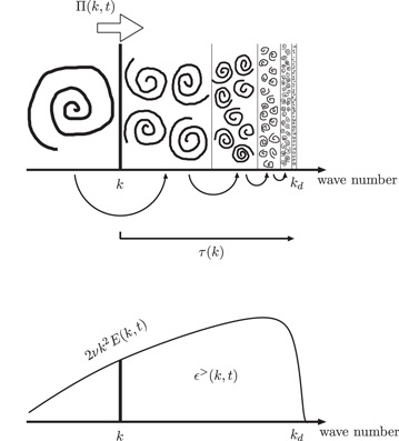
Figure I.2-10: The local equilibrium hypothesis [13].
Kolmogorov’s hypothesis and findings are still widely used in fluid mechanics and turbulent flow descriptions as they quantify the relationship between large and small vortices, which was already observed and expected by Da Vinci and Richardson.
Even if these findings and theories provided sets of equations which could, in theory, be solved in order to obtain a complete understanding of a turbulent flow, their complexity and heavy computational cost - as already hinted by Richardson – still were a limiting factor.
These inconveniences would only be coped with later, thanks to a new breakthrough: the computer age.
Von Kármán vortex street experiment [6]
Turbulence in the Computer Age
“Perhaps some day in the dim future it will be possible to advance the computations faster than the weather advances and at a cost less than the saving to mankind due to the information gained. But that is a dream [5].”
When this quote was made in 1922, the term "computer" did not refer yet to a powerful machine capable of processing a large amount of data, but rather to a human, performing calculations by hand using instruments such as calculating machines or mathematical tables. The experimental capabilities were limited, and the idea of machines running numerical simulations was unthinkable. Since then, considerable progress has been accomplished. The introduction of electronic computers has brought significant advances in the study of turbulence by revolutionizing scientific research. Indeed, computer simulations remarkably enhanced experimentation. Direct Numerical Simulation (DNS) of turbulent flows is a good illustration of the achieved breakthrough. However, a long process has taken place before such a progress became possible.
Pioneering ideas
Before the computational approach became such a turning point, three men were already ahead of their time: Poincaré, Taylor, and Richardson [33]. Each of them noticed something that would only be explored in-depth many years later.
At the beginning of 20th century Jules Henry Poincaré first recognised that a system of three deterministic equations can lead to random-like behaviour, by solving the “three body problem”, which describes the movements in space of the Earth, Moon and Sun under their mutual gravitational attraction [44]. In particular he introduced the concept of sensitivity to initial conditions, described in “Science et méthode” [45]. When talking about the “hasard”, he defines it as a very small and therefore unpredictable change of conditions, such that it influences the result. Therefore, even if someone perfectly knows the laws governing a given phenomenon, he will never be able to know perfectly and exactly the initial conditions, so the predictions will never be totally reliable, since a small change in the initial conditions can give very different results. Even if his discovery of deterministic chaos was a breakthrough in the common resolution of deterministic equations, it had no impact on science, until the development of the computational numerical simulation allowed a detailed study of the so called “deterministic chaos”.
Nearly one decade later, in 1921, Taylor provided an exact Lagrangian solution for the rate of spread of tracer in unbounded, stationary homogeneous turbulence, giving birth to the Lagrangian perspective on turbulent dispersion. Taylor’s result may easily be obtained by an analysis of Langevin’s equation, which had been developed to describe Brownian motion and represents “the first example of a stochastic differential equation” [38]. Taylor’s result has served to guide turbulent dispersion modelling, however, its adequate extension to inhomogeneous and nonstationary turbulence, in the form of today’s Lagrangian stochastic models, occurred only after newfound access to computers spurred heuristic experiments in the numerical simulation of particle trajectories.
Around the same time, Lewis Fry Richardson, who has contributed to important results in meteorology but also in numerical analysis and fluid dynamics, took a great interest in weather prediction. He had very innovative ideas. However, they were quite impractical due to the lack of computing tools, which lead him to make the quote introducing this section in 1922, after his unsuccessful attempt to make a weather forecast. To set the context that elicited that belief, it is necessary to understand his experiment. He introduced the idea that the evolution of atmosphere is ruled by equations and that if the initial conditions are known, numerically integrating the equations is sufficient to determine the future weather. Strengthened by this conviction, he wanted to try his assumption and chose as an initial condition a record of the weather conditions observed in Northern Europe at 4 a.m. on May, 20 1910 during an international balloon day. He started the long and tedious task of trying to predict the weather, utilizing some rudimentary computing machine and making all his calculations by hand. He worked for at least 100 hours in the course of two years, only to obtain disappointing results [33]. He came to the conclusion that the atmosphere is complicated and that more people are required to make the calculations to get a more accurate prediction. He envisioned a kind of factory made of 64000 human computers who will calculate by hand the weather forecast (Figure I.3-1). This was a pioneering idea depicting in the earliest times the concept of parallel computers.
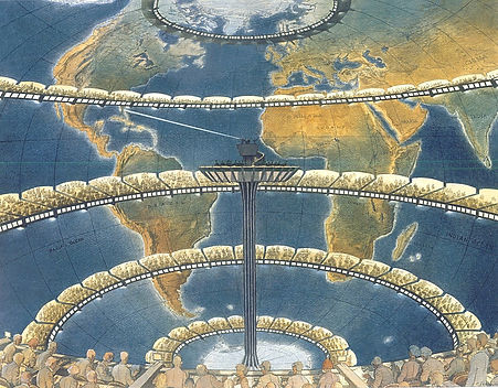
Figure I.3-1: Richardson's Forecast Factory (© F. Schuiten [31])
Computational efforts
An increasing interest towards computing machines started twenty years later, in the 1940s, when the first electronic computer was used by Los Alamos National Laboratory to study finite-difference methods for solving partial differential equations. But the research was restricted only to atomic weapon system development and wartime technology [34] for the Manhattan Project. The transfer of ENIAC (Electronic Numerical Integrator And Computer) in Aberdeen in 1947 was an important turning point for fluid dynamics, expanding the applications of computer simulations from only military purposes to scientific research. A leading figure in the Manhattan Project, John von Neumann, recognized the importance of computers for the study of turbulence, in a 1949 review, anticipating already the direct numerical simulation (DNS) of turbulent flows:
These considerations justify the view that a considerable mathematical effort toward a detailed understanding of the mechanism of turbulence is called for. The entire experience with the subject indicates that the purely analytical approach is beset with difficulties, which at this moment are still prohibitive. […] Under these conditions there might be some hope to ’break the deadlock’ by extensive, well-planned, computational efforts [29].
Although the computers greatly helped in advancing the research, at that time, they did not benefit yet from very powerful computers, which somehow limited the number of representative calculations they could conduct in an investigation.
Furthermore, concerning the development of Lagrangian stochastic models, it was not until computers became accessible to meteorological offices and universities in the 1960s, that atmospheric dispersion was approached along Lagrangian lines as realistic atmospheric turbulence.
Deterministic chaos
Despite the contributions of Poincaré at the end of the 19th century, the development of the deterministic approach in science is due to the computational efforts made starting from the 1940s and culminated with the work of Edward Norton Lorenz, “Determinisic Nonperiodic Flow” [46].
It is inspired from his personal experience; in fact, he was a MIT meteorologist and in 1961 he was working with a computer for investigating the models of atmosphere, which contained twelve differential equations. The computer was working with an accuracy of six decimals, but once he decided to give only three decimals of the initial values, and then went for a coffee. When he returned back he found that the results were significantly different from the ones previously calculated. So, he has rediscovered what has already been affirmed by Poincaré, i.e. the sensitivity of the system to the initial conditions. Lorenz then published his conclusions in [46], where he analysed the models of hot air raising in atmosphere when close to a hot surface (in a case with high Rayleigh number, i.e. with pure convection). This problem is governed by a system of three non-linear differential equations (the same type of equations previously solved by Poincaré), reported in Equation 1, where X, Y, Z are the variables, X’, Y’ and Z’ their derivatives, and σ, b and r are parameters, which are kept constant in the simulation.

Equation I.3-1: System of differential equations solved by Lorenz in [46].
Lorenz obtained the numerical solution of the problem through a computational simulation, and the results were graphically represented in Figure I.3-2, where the so-called Lorenz attractor or strange attractor is illustrated. The system of equations had three unstable equilibrium solutions, so that all the solutions, represented in the state space, are “attracted” by these points, but they never pass through them. So, if a solution is computed starting from a more or less random initial point, it will describe oscillations around the three points; the oscillations around one stationary point increase in amplitude and when the critical size is reached, they start oscillating around one of the other points. Therefore it can be noted that the solutions are all contained within the same boundaries, but are nevertheless aperiodic and sensitive to initial conditions.
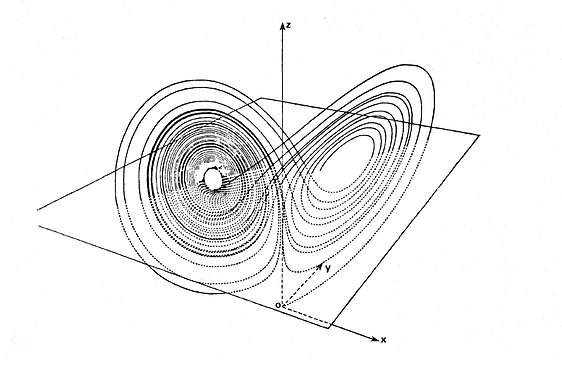
Figure I.3-2: Lorenz’s attractor (Modified from [24]).
Lorenz then concluded his study by saying that when these concepts are applied to meteorology, which has always been considered as non-periodic, they lead to the impossibility of predicting the climate over a long period of time, as the solutions diverge from each other at an exponential rate. Lorenz's contribution made him worldwide known as the father of chaos theory.
Even if his studies were not focused on turbulence, Lorenz had a great impact also on this field. In fact, he underlined how the variation of one parameter in a system of non-linear differential equations can lead to a transition from periodic to non-periodic conditions. The same transition from a regular situation to an irregular one is possible for any system of non-linear differential equations, so it is also valid for the Navier-Stokes equations, where a transition from laminar to turbulent behaviour might occur.
The same concept had already been developed by Reynolds with his parameter: a change in the Reynolds number leads to a bifurcation, i.e. a transition from a steady state to a turbulent one, which can be represented as a strange attractor. The studies on the transition brought to the introduction of the so-called “bifurcation theory”, that was worked out by Ruelle and Takens [47], Pomeau and Manneville [48] and Landau and Hopf [49].
In [47], the flow behaviour when increasing the bifurcation parameter is studied and brings to the following bifurcation sequence:
Steady → Periodic → Quasi-periodic → Chaotic
Another possible sequence is reported by Pomeau and Manneville in [48], where the concept of “intermittency” is introduced. In fact, when increasing the bifurcation parameter, there might be events of finite duration, called “bursts”, that take the solution away from the regular ones. The frequency of the “bursts” increases with the bifurcation parameter, so that at the end the periodic behaviour is no longer observable, thus leading to a chaotic motion. So, the sequence reported by [48] is the following:
Steady → Periodic → Intermittent → Chaotic
The above presented bifurcation theories were in contrast with the Landau-Hopf one, which was developed in 1940s separately by Landau and Hopf [49]. They supposed that the onset of turbulence is due to infinite transitions that increase the instability of the flow. The Landau-Hopf bifurcation theory is still used today as an important methodology to study turbulence.
Lagragian stochastic modelling
As mentioned above, the development of the Lagrangian perspective on turbulent dispersion started in 1921 with Taylor.
The aim of a Lagrangian stochastic (LS) model is to calculate the paths of a large number of individual particles through a turbulent flow as they travel with the local wind field, based on knowledge of velocity statistics. These three-dimensional models allow us to explain flow and turbulence space-time variations [40].
Emissions in the atmosphere are simulated using a certain number of fictitious particles named “computer particles”. Each particle represents a specified pollutant mass. It is assumed that particles passively follow the turbulent motion of air masses in which they are, thus it is possible to reconstruct the emitted mass concentration from their space distribution at a particular time. The reference system moves with the particles, as shown in Figure I.3-3.
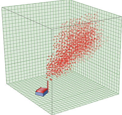
Figure I.3-3: reference volume enclosing the computer particles of pollutant [39].
The simplest class of LS model is the random displacement model, (or zeroth-order LS model), which represents a particle trajectory by a sequence of random increments in position. The more sophisticated is the first-order LS model that creates the particle path by integrating a sequence of random increments in velocity., such that the particle position X and velocity U together constitute a Markovian state variable (a Markov model is a stochastic model used to model randomly changing systems, assuming that future states depend only on the current state, not on the events that occurred before it).
The fundamental advantages of a “first-order” Lagrangian stochastic model relative to alternative descriptions of turbulent dispersion are, on the one hand, its ability to correctly describe the concentration field and, on the other hand, its ability to rationally incorporate all available statistical information on the velocity field.
By the late 1960s, access to digital computers had penetrated to the level of meteorological offices and universities with many attempts to numerically mimic atmospheric dispersion as realistic atmospheric turbulence with the Lagrangian approach. Thompson suggested that in treating atmospheric dispersion problems, rather than adopting a “deterministic method”, “it may often be more useful to simulate the original physical situation directly” and that doing so “also turns out to be simpler.”
The span of applications of the modern Lagrangian stochastic model can be illustrated by its capability of tracking particle motion throughout and even above the troposphere, from one continent to another, by being coupled to flow fields calculated by numerical weather prediction models. An important motivation for the development of these models was the Chernobyl reactor accident in 1986, which highlighted the need to be able to estimate long-range transport and dispersion in a timely and flexible way. These types of models are now used to estimate the dispersion of a wide variety of materials including radionuclides, chemicals, volcanic ash, airborne diseases, and mineral dust. Another more recent catastrophe which led to fluid dispersion calculations of this kind was the Refugio oil spill in 2015 in Santa Barbara County, California, which deposited tens of thousands of U.S gallons of crude oil onto the west coast, due to the rupture of a pipeline. Immediately after the incident, oil samples were taken and data was gathered, which allowed to predict in what directions the oil might spread after calculations of velocity streams [43].
In a nutshell, the Lagrangian stochastic models of dispersion has matured, but there remains room for fundamental progress. These models are being used with success on scales from the individual farmer’s field or the city block, to the intercontinental, and indeed, they have assumed a vital social role, nicely exemplified by their application to predict the hazards of volcanic ash clouds [41] or to locate or quantify sources of air pollutants or greenhouse gases [42].
Milestones in computational turbulence
In 1970, a landmark decision was taken by Dean Chapman, the director of Aeronautical Science Directorate of the NASA Ames Research Center at that time. He created the Computational Fluid Dynamics Branch which was the first coherent and structured CFD organization for aerodynamic application [34]. It gathered talented experts devoted to purely numerical work and collaborating together to promote knowledge, excellence and hard work. One of the challenges consisted in upgrading the computational facilities. Around that time, Seymour Cray [36], the father of supercomputing, contributed to bolster the research by making high-speed computers commercially available, such as CDC 6400 and CDC 7600 (Figure I.3-4). And in that infrastructure where talented experts supported by powerful machines could carry out their work together, the CFD research has experienced a spectacular development.
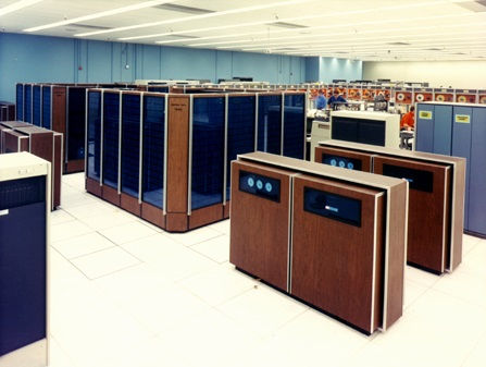
Figure I.3-4: Lawrence Livermore National Laboratory; CDC 7600 (© Gwen Bell [80])
But even with all this infrastructure, the turbulence problem remains the Achille's heel of CFD. It is worth recalling that at the very beginning of CFD, solving the time-dependent Navier-Stokes equation was the main concern. However, it is a complex task. Among the early milestones in CFD, we can cite the multi-grid method introduced by Brandt [28], achieving a fast convergence rate of an iterative approach to a steady- state asymptote for the Navier–Stokes equations. Shortly after, massively parallel computing technology coupled with load balancing marked a major step forward by providing enhanced performance.
Turbulence research really blossomed in the 1970s, with the most notable success being the development of numerical schemes, computational techniques and hardware to study turbulence. The first one was the Large Eddy Simulation (LES) proposed in 1970, followed by the Direct Numerical Simulation (DNS) in 1972, and the introduction of Reynolds-averaged Navier–Stokes (RANS) approaches also around 1972 [15]. An overview of these approaches is given in Figure I.3-5:
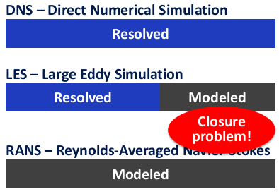
Figure I.3-5: Three levels of simulation [14].
The Direct Numerical Simulation (DNS) approach has been revolutionary in its impact on turbulence research because of the ability to simulate and display the full three-dimensional velocity field at increasingly large Re, which is practical to study the structures of the flow and correlate them with turbulent transfer processes. Direct Numerical Simulations are aimed to run on supercomputers as no closure or sub grid approximations are used to simplify the flow. The flow follows all the motions of the full-blown Navier-Stokes equations at large Re. The first DNS in 1972 had a resolution corresponding to Re≈100, then Re≈6000 was reached in the early 1990s [35], and Re~105 in the early 2000s [30], which is approaching fully developed turbulence in modestly sized wings. The DNS approach key strength resides in the fact that it can resolve all the scales of motion accurately. Nevertheless, it is highly expensive and the amount of computer resources required to solve all scales of three-dimensional motion is challenging. For instance, the flow around a car have a too wide range of scales to be directly computed using DNS. Therefore, instead of direct simulation, a simpler description through a statistical modeling approach and averaging can be taken.
The Reynolds-averaged Navier- Stokes (RANS) approach is a non-expensive alternative to DNS. In fact, the approach taken is the opposite of DNS. Nearly all scales of solution are modeled and only mean quantities are directly computed [15]. However, as a model, it suffers from the closure problem. Indeed, the first priority of this approach was to provide computational efficiency, rather than getting a fully accurate representation of turbulence. For the RANS engineering model, an infinite set of equations for higher order moments is required. However, computers cannot solve a system of an infinite number of equations. One needs to close the set at a small number to have computational efficiency. At any stage of approximation, undetermined coefficients are set by comparison with experimental or DNS (Direct Numerical Simulation) data.
The Large Eddy Simulation (LES) approach [37] is a compromise between the traditional RANS methodology and the computationally expensive DNS approach. The main idea consists in resolving only the large eddies containing information about the geometry and dynamics of the flow. The influence of the small scales is approximated with the subgrid model. The subgrid-scale model (SGS) allows to mimic the drain of the energy cascade by removing energy from the resolved scales. However, as a modeling approach the LES approach also suffers from the closure problem.
It can be established that each type of computational simulation has contributed to the understanding -and therefore in the controlling- of turbulence, from meteorology studies to the dispersion of pollutants through a turbulent flow. The computational models described in this section will be the first tools required for actuating on turbulent flows, which is essential in some engineering applications, as it will be shown in the next section.
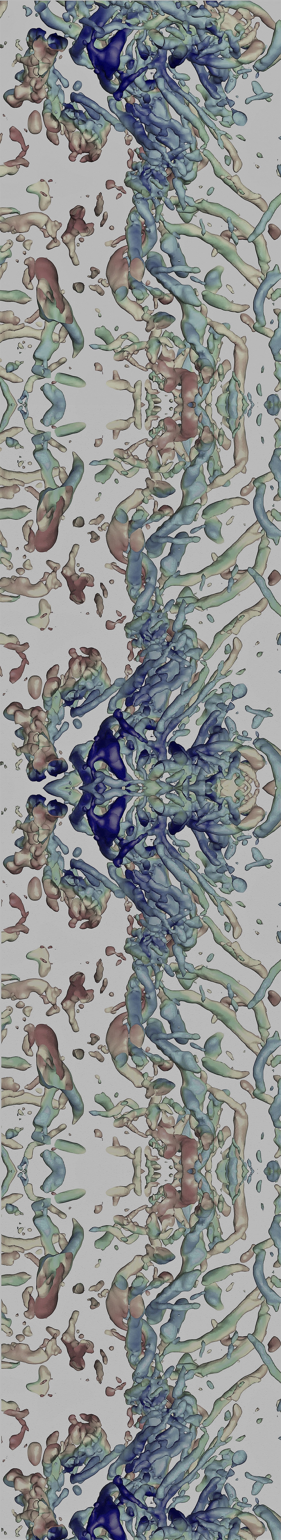
Lagrangian tracks color coded in a homogeneous isotropic turbulence [87]
Impact

Controlling Turbulence
As it was apparent in the previous sections of this blog, turbulence is nowadays more than ever a multidisciplinary field that, through the centuries, brought together many scientific communities.
Because of its versatile nature, turbulence was either a source of inspiration or labour for engineers as well. It has played a role in many scientific innovations from different fields, even when it was least expected, thus, making this puzzling phenomenon even more interesting to the engineering community. This section therefore provides a taste of what are the main fields, challenges and discoveries related to turbulence control.
Turbulence as scientific vs. engineering problem. Active and passive control.
As it has already been mentioned in section I-1.1 The discoveries of Da Vinci, two aspects from da Vinci’s observations are still valid which underpin many engineering models of turbulence and scientists investigating the role of these structures as "the possible of turbulent dynamics [3]".
Engineers developed methods to get accurate results with minimal computational effort trough making simple models for the effects of turbulence and adjusting coefficients in the model by fitting computational results to experimental data. There are many fields that have benefited from reliable data, for instance, aircraft design and aerodynamic drag reduction for automobiles to achieve better fuel efficiency, a theme that will be further investigated in the blog. The main goal of many engineering models —as the Lagrangian Stochastic model described in the Turbulence in the computer age section— is to estimate transport properties—not just the net transport of energy and momentum by a single fluid but the transport of matter such as pollutants in the atmosphere or the mixing of one material with another.
For many engineering applications such as car aerodynamics, in order to improve the speed of a vehicle through drag reduction, it is necessary to modify locally the flow, to remove or delay the separation position, or to reduce the development of the recirculation zone at the back and of the separated swirling structures. This can be mainly obtained by controlling the flow near the wall with or without additional energy using active or passive devices. Significant results can be obtained using simple techniques. For instance, as described in [55], flow control is obtained when the wall pressure distribution is successfully modified near a car’s rear window and back, using various adapted devices which change locally the profile’s geometry. Control experiments in wind tunnel on reduced or real ground vehicles are performed and measurements of the wall static pressures and of the aerodynamic torque allow to quantify the influence of flow control [56]. However, due to the design constraints, the real gain is rather weak and so new control techniques must be developed. Among these new techniques currently investigated by the engineering and scientific communities, separate devices located in front of or behind the vehicle can be used to reduce the development of the recirculation zone on the rear window or at the back and the interactions of the swirling wake structures [54].
Sensing and actuating
Historically, studies of turbulence have progressed through advances in experimental measurements, theoretical descriptions and the introduction of numerical simulation of turbulence on high-speed computers. But what were the main fields and applications that really drove its investigation?In the early to mid-20th century,turbulence researchers were motivated by two important practical problems: predicting the weather and building very sophisticated aeroplanes. Aircraft development led to the construction of large wind tunnels, where measurements of the drag and lift forces on scaled model aircraft were used in the design of airplanes (See on Figure II.1-1 the now world famous and textbook-knowledge wind profile lift-drag diagram [3]).
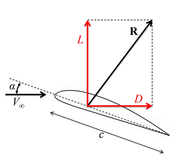
Figure II.1-1: Aerodynamic forces lift “L” and drag “D” defined with respect to free stream velocity V∞.(Credit:V.E. Terrapon [14]).
In order to gain some insight on their impact, such improvements and technologies were necessarily associated to measurement and sensing systems. Relative flow velocity has usually been quantified through vanes and differential pressure measurements. Such meteorological applications have historically required large multi-engine airplanes to accommodate on-board computers, instrumentation and system operators. The large size and high speed of these airplanes also greatly increase the flow disturbance. Their airframes present a large obstruction to the flow around them, while their weight requires a major flow distortion to remain airborne. Because of this, and the need for frequent and tedious calibration, vanes have been replaced by the more robust pressure spheres that have the advantage of not interfering with storm avoidance or research radar in the nose of the complex aircraft.
This pressure sphere approach has three interesting features: co-location of all high-frequency motion sensors within a small pressure sphere, measurement of the temperature at the central port of the pressure sphere and measurement of static pressure from ports directly on the pressure sphere. Thus, nearly all sensors necessary for atmospheric flux measurement by eddy correlation have been located within a small package. The latter, with minimal modification to the airframe, may be extended into undisturbed air. Compact pressure sensors, mounted inside the pressure sphere, eliminate long pneumatic connections.
Unfortunately, this configuration measures turbulence directly on the body of the aircraft, in the disturbed flow, which requires potentially complex individual calibrations for each installation. Also, for negative attack angles, desirable calibrations in flight are not possible. Only if the probe is in undisturbed air can the positive-attack calibration coefficient, observed in flight, be freely extrapolated to negative attack angles. Thus, a slower airplane has evident advantages and the current probe is designed for airplanes flying at half the airspeed of most existing systems [57].
Is turbulence only a high-and large-scale phenomenon? Interest and motivation of small-scale turbulence
In the last few decades, scientists turned their interest to a new field of fluid dynamics that observes flows that occur at a microscopic scale. Among the many reasons for which such length scales attract the scientific community, the downscaling of processes allowed to reduce the cost, the processing time and the quantities of the reagents needed for many biochemical analyses [51].
Microfluidics is a particularly interesting field, as in this context, turbulence is sought rather than avoided. Indeed, because the forces involved at these scales are different than the ones encountered in macroflows, the dynamics of such fluids is different and so are the main governing processes involved.
For instance, in the macroworld, mixing is primarily governed by turbulent and convective motion. Indeed, when pouring a splash of milk in a cup of coffee, the mixing would take an unbearable amount of time if the cup was left as it is, it is really the additional spoon motion that will in turn, lead to an efficient mix. In the microworld, and in particular, in a microfluidic channel, mixing is primarily governed by diffusion, which can be efficient when the distances that need to be unravelled are short, see Figure II.1-2. Even if the flow speed in the microchannels can be high, laminar conditions are almost always encountered due to the small considered length scale, leading to a low Reynolds number.

Figure II.1-2: Convective mixing in a cup of coffe (Credit: C. Ma, Flickr [81]).
Nonetheless, when the chip’s characteristic dimensions and the microchannel travelling time are limited, diffusion might not be enough to provide complete mixing of the reagents. In that case, one may want to enhance mixing by establishing a turbulent regime in the microfluidic chip.
In order to create turbulence, one needs to counter the strong viscous forces acting on a laminar flow and thus, an additional body force can be introduced as defined in Navier-Stokes equations. Previous work, such as [52], attempted to induce electrokinetic mixing by applying electric fields to a conductive flow. However, the obtained improved mixing was a result of laminar chaos, not turbulence.
Instead, in [50], a novel approach for designing an elektrokinetic mixing chip, able to produce a turbulent flow, is described (Represented on Figure II.1-3(a)). This design induces a non-uniform electric field that acts on two conductive solutions that are dyed with a fluorescent marker for imaging purposes.

Figure II.1-3: Laser-induced fluorescence of the mixing process in the microchannel. Credit: G.R. Wang et al., University of South Carolina [50].
If the viscous, inertial and electric forces are balanced with an electric field, the smallest motion length scale is smaller than the channel dimensions for a high value of the electric field and conductivity difference. Therefore, with an adequate set of electrical parameters, a characteristic small scale can be reached, leaving room for a multi-scale phenomenon, one of the main characteristics of a turbulent flow. A priori, the electrical parameters therefore provide a complete control over the turbulent features.
Small-scale turbulence observation and quantification
Figure II.1-3(b)shows a fluorescent picture of the channel with the two reagents flowing freely, that is, without any electrokinetic forcing. The two liquid layers only mix at their interface due to diffusion, but the two phases remain quite distinct over the represented section of about 500[µm].
Forcing is then successively applied and the effect of an increasing electric field can be seen on Figures II.1-3(c) and (d). In these forced situations, mixing becomes rapid (up to 1000 times faster than the purely diffusive case, according to [50] and efficient. In particular, vortices mix the two liquids even close to the inlet where they encounter on Figure II.1-3(d).
Streamlines can be observed by inserting particle tracers in the flow conditions of Figures II.1-3(b) and (d). The obtained fluorescence images are shown on Figures II.1-3(e) and (f), where the particles undergo a laminar motion on the former and a turbulent and chaotic one on the latter.
One of the main challenges encountered by the authors was to quantify turbulence on the microfluidic chip. This part of their work was crucial. Indeed, as it was mentioned in the previous section, turbulence measurement and quantification are usually a key element in turbulence control.
At the considered length scales, probes and intrusive speed or vorticity measurements can completely disrupt the flow. The authors therefore used a laser-induced fluorescent non-invasive imaging technique with a high spatial resolution [53].
This particle tracing system allowed measurements of local flow speed, fluctuations, turbulent energy and power spectrum density. All of these are analysed and presented by the authors with ranging values of the applied electric field, allowing the main features of the flow to be observed and quantified: efficient mixing, high dissipation, irregularity, multi-scale eddies, 3D features and continuity. Despite low Reynolds number in the microchannel, all these features are characteristic of a turbulent flow, as described in [15].
Overall, turbulence was not only achieved in a microfluidic chip, but was also quantified through non-invasive imaging techniques. These two innovations are revolutionary, not only because they occurred in a low Reynolds context, but also in terms of perspective regarding efficient mixing, flow control and measurement in microfluidics. The appearance of turbulence in a situation where it was least expected shows that the understanding of this complex phenomenon is still limited. However, discoveries such as the ones described in this section provide interesting opportunities and perspectives that may involve many other scientific fields that have not been considered until now.
This entire section and the results highlighted throughout it underline the fact that quantification and control of turbulence are tedious tasks that can, however, provide major breakthroughs and innovations in terms of engineering applications and technological impacts, ranging from the tiniest microfluidic flow, to the planetary air flows involved in weather phenomena. Advances in experimental measurements of turbulence were mostly driven by the massive efforts and interests raised by Aerodynamics. The contributions of turbulence study to this field will be explored in the next section, along with a discussion on approaches used to counter turbulence in distribution networks.
Flow of complex fluids through microfluidic channels [88]

Aerodynamics and Distribution Networks
Aerodynamics is one of the major contributors to the advances in turbulence study. In this field where interest keeps growing, special attention is paid to turbulence research. But turbulence also triggers the interest of other industries, such as distribution networks, to name but one example. This section will present the impact of turbulence on aircraft design with a focus on drag reduction, followed by a research project pointing out methods to counter turbulence in pipe flows.
Aerodynamics
Drag forces are at the heart of aerodynamics. Their complexity and importance govern the design of planes, boats, rockets and shuttles. The designers secretly hope for negative drag but the subject is tricky and controversial [62]. In aerodynamic design studies, drag is directly linked to the aircraft weight needed to carry a specified load. These parameters determine the economic viability of an aircraft manufacturer, aiming at drag minimization associated to safety and comfort maximization.
Moreover, the environmental factors, such as noise, air pollution and the future growth of the civil aviation will have a negative impact on environment. Therefore, new technologies are becoming increasingly paramount in order to reduce drag and consequently the fuel consumption and CO2 emissions.
The total drag force in a civil transport aircraft is mainly composed by the skin friction drag and lift-induced drag. The skin friction drag is a consequence of a plane’s shape and is more significant at cruise speeds. The lift-induced drag is more dominant during take-off and landing. It has the origin on the tip vortex generated when air moves at different speeds over the top and bottom of the wing, as shown in Figure II.2-1.
Figure II.2-1: Lift-induced drag acting in an aircraft (Mecaflux Helicel, 2018 [82])
There are two methods generally considered for skin friction drag reduction. The first one aims at reducing the turbulent skin friction while the second one aims at delaying the turbulent transition to maintain large extent of laminar flow.
During a flight at high Reynold numbers is difficult to maintain laminar conditions. Therefore, turbulence drag must be mitigated. In order to do that, riblets, represented in Figure II.2-2, and large Eddy Break-Up Devices, represented in Figure II.2-3 are used to limit the development of large eddies in the boundary layer. Another way for achieve drag reduction is the use of vortex generators, shown in Figure II.2-4, to improve the boundary layer’s resistance to separation.

Figure II.2-2: Riblet geometries and their reduction in wall friction of a turbulent flow [64].
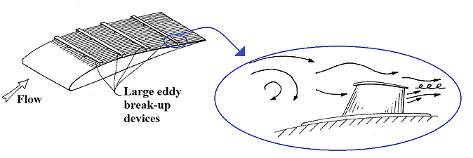
Figure II.2-3: Eddy break-up devices in aircraft wing
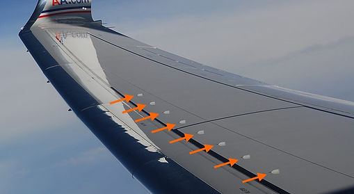
Figure II.2-4: Vortex generators in a wing of a Boeing 737-800 [83].
An emerging drag reduction technology is the “smart surface”. It was inspired by sharks, as their skin self-adjusts with the flow. This method consists in a composite surface that combines riblets with an elastic coating that also changes its form due the nature of the flow, as represented in Figure II.2-5.
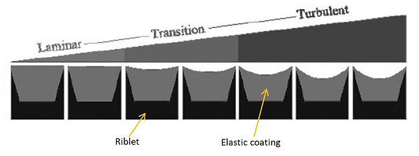
Figure II.2-5: Smart surface [62]
The most common method used to decrease the lift-induced drag consists in increasing the aspect ratio of the wing. However, the latter is a compromise between aerodynamics and the structure characteristics themselves, and it is clear that for a given technology it is not always feasible to increase aspect ratios. The alternative is to develop wing tip devices to reduce the wake vortex as shown in Figure II.2-6. By cutting the vortex and drag, the aircraft uses less fuel to achieve the same results.
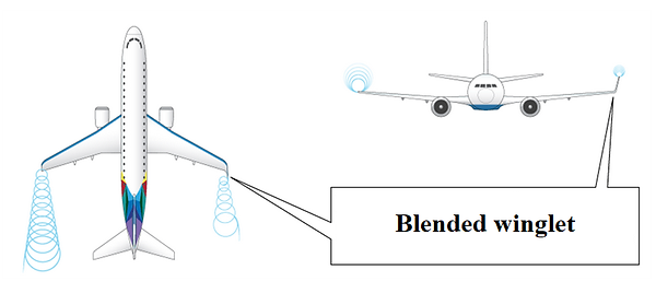
Figure II.2-6: Wing tip device: the effect of a blended winglet when compared with a conventional wing [84].
Drag reduction has motivated aerodynamics during the years, allowing drastic performance improvements in planes, as represented in Figure II.2-7. Turbulence descriptions and understanding allowed push forward the technologies involved in drag reduction. Adding the help of software to run simulations, the scientists can now better understand the behavior of the airfoils that they build. Improvements in turbulence studies will further push the development of new technologies, such as the X-43A scramjet that will possibly go around the world in only a few hours.
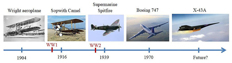
Figure II.2-7: Aircraft development from Wright brothers, crossing the two world wars and the expectations for the future.
Distribution networks
Turbulence has a significant impact on distribution networks, especially on pipe flows. The phenomenon is responsible of friction losses which cause a severe drag increase that needs to be countered by employing large forces. Nowadays, it is estimated that nothing less than 10% of the global energy consumption is used to achieve this task [58].
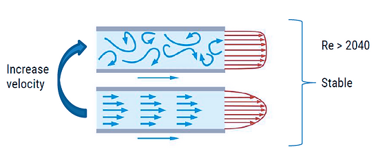
Figure II.2-8: Illustration of how a laminar flow goes to fully turbulent by increasing the velocity
Industry has developed several strategies to counter turbulence via feedback mechanisms that only focus on one component of the velocity field [59] (implies that we know it in details) or via active and passive methods that are not that efficient to use in real life because their costs are higher than the gain obtained by the drag reduction.
Instead of focusing on one component of the velocity field, changes can be applied to the mean velocity profile in order to make the turbulent flow re-laminarized.
Using Direct Numerical Simulation, it could be demonstrated that under some ideal conditions, flows at a high Reynolds number can return to a laminar state while perturbing the mean profile. On the experiments recently performed, one makes a Direct Numerical Simulation by injecting a laminar flow into a pipe, perturbing it to make it become turbulent and then rescales it by a certain factor.
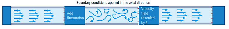
Figure II.2-9: On a pipe with boundary conditions applied in the axial direction, one can rescale a turbulent velocity field by k to make it returns to a laminar state.
The rescaling can be performed using original ways, such as placing rotors downstream, having a portion of the pipe pierced by 25 holes in where a fluid is injected or just injecting a fluid in the stream wise direction, which increases the wall shear stress and causes the deceleration of the flow in the pipe center [60].

Figure II.2-10: First experiment. 4 rotors are set downstream and act as the rescale module. The abrupt change leads to a complete laminar fluid until the end of the path.
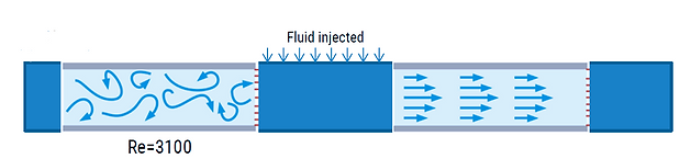
Figure II.2-11: Second experiment. Fluid is injected through 25 holes in a portion of the pipe. The injection creates counter rotating vortices that act as a rescale module. These vortices lead to a flattened velocity field profile and the flow returns to laminar until the end of the pipe (NB: the quantity of injected fluid is an tiny fraction of the total fluid flowing through the pipe [58])
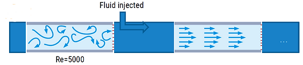
Figure II.2-12: Third experiment. Fluid is injected in the stream wise direction, augmenting the wall shear stress leading to a lower velocity of the fluid in the central part of the pipe. This reduces the mean velocity field and leads to a laminar flow until the end of the pipe.
Perturbing the mean velocity field with such techniques leads to a power saving up to 55%, and the flow remains laminar until the end of the path. One can also think that given all those techniques imply a local change to the velocity field; a global modification could also be applied.
On the Direct Numerical Simulation, a forcing term can be added in the Navier-Stokes equations in order to test a connection between the initial flat velocity profile and the subsequent turbulence collapse. Note that this forcing term is applied globally.

Figure II.2-13: A moving part is added to the pipe, in order to apply a "forcing term" globally. This leads to an increasing of the wall shear stress resulting in a deceleration of the flow like in Figure II.2-12. This leads to a flattened velocity field and it remains laminar until the end of the path.
Recent experiments showed that when setting a moving part to a pipe, which is 4% larger than the rest of the pipe and that moves in the stream wise direction, an energy gain of 90% can be obtained. In fact, the impulsive acceleration of the near-wall fluid lead to a flattened velocity profile which brings to a laminar velocity field.
As it has been demonstrated, one of the major technological problems of the world can be solved using the intuitions given by the computer simulations. In fact, a power saving of 90% could be achieved, which mean that only 1% of the global energy consumption could be used for counter turbulence in distribution networks. So, the remaining 9% could be saved or used for honorable causes. The methods above are simpler than the ones that already exists that are only based on one component of the velocity field, because a full knowledge of the velocity field is not required as changes are applied to the mean velocity field.
Thanks to turbulence study, tremendous progress has been made in aerodynamics as well as in distribution networks. However, only a subset of the countless achievements has been mentioned. There is still much more to introduce. Following this idea, next section will enforce the influence of turbulence study on mixing, dispersion and energy harvesting.
Water distribution network [89]

Mixing, Dispersing and Energy Harvesting
An application of turbulence research that focuses on countering turbulence was introduced previously. In this section, rather than trying to eliminate turbulence, the effort will be directed towards trying to gain a better understanding of turbulence. This will enable the creation of better designs to put up with turbulent flows or even better, to benefit from them. Indeed, turbulence can be used as a means to enhance mixing. Understanding how this complex phenomenon affects the dispersion of air pollution and energy harvesting allows to improve the design of cityscapes and wind turbines.
Mixing
Mixing is a process aimed at the reduction of inhomogeneity in a physical system, both in terms of concentration, phase or temperature [67]. Several examples of mixing in daily's life can be found, in fact like Monsieur Jourdain says in Moliere’s play (1670), all of us “do mixing without even knowing it” [68]. One of the well-known characteristics of turbulence is its capacity to enhance mixing, and this aspect is exploited by several industrial applications. In process engineering, for example, it is one of the key parameters for achieving the desired product quality. However, it is not always possible to guarantee homogeneous conditions in a chemical reactor, especially for large scale processes. Indeed, this consists in the main issue encountered when trying to scale-up a process (Figure II.3-1), namely when enlarging it so that the production is increased.

Figure II.3-1: Scale up sequence for a biological process from laboratory to industrial scale [69].
Several correlations are available for scaling-up a process and for evaluating the mixing properties, but in most of the cases they are not enough for describing the phenomena that occur at large scales. Because of this inadequate understanding of mixing processes, economic optimisation cannot be performed, and in 1989 it was estimated that because of the lack in mixing information has caused an additional expenditure to USA industries between 1 and 10 billion $ per year [67].
However, thanks to the development of the turbulence models as well as the advancement in CFD simulations, several configurations of industrial interest can now be modeled, and the results can be compared to experimental studies. Since several solid-liquid chemical processes, such as catalytic reactions, crystallization and polymerisation, are performed in stirred solid-liquid reactors (Figure II.3-2), many research efforts have been devoted to this subject, in order to understand how the solid phase influences mixing.
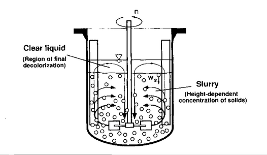
Figure II.3-2: Stirred solid-liquid reactor [71].
This subsection presents the work of Kasat et al. [70], where a stirred solid-liquid reactor is simulated thanks to FLUENT 6.2 software, where RANS equations with the Boussinesq’s hypothesis are used, and the eddy viscosity is defined with the k-ε turbulence model. The results in terms of mixing time are reported in Figure II.3-3, where three zones are clearly identifiable, depending on stirrer speed:
-
If the speed is low, then the particles are not suspended in the reactor, so the solid does not cause any difference in the mixing time;
-
If the speed is large enough to suspend the particles and create a slurry, then the mixing time increases up to a maximum value. This is due to the fact that the distribution of the particles in the reactor is irregular and the presence of the solid reduces the flow velocity and therefore increases the mixing time, especially in the highest zone, where only the liquid is present, and which corresponds to the last zone where the homogeneous conditions are reached;
-
After the maximum value of the mixing time an increase of the stirrer speed leads to a decrease of the mixing time, until it returns equal to the monophasic case.
So, depending on the achievable rotational speed of the process, the relative mixing time can be evaluated.

Figure II.3-3: Mixing time variation as a function of rotational speed [70].
Moreover, studies like [70] are used as comparison with experimental studies performed under the same conditions. In this case the model results are confronted with the experimental results obtained in [72]. As it is shown in Figure II.3-4, the results of the two analyses are quite similar, and this gives a validation to the CFD model, since it is able to represent the reality of the problem.
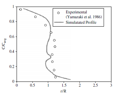
Mixing is only one of the multiple ways of industrially exploit and control turbulence; other interesting examples of such application are presented in the following sections.
Dispersing
Along with mixing, dispersion is one of the main topics of interests in turbulence study. Dispersion is principally explored in environmental flows where turbulence plays an important role on the emission of pollutants. Computational Fluid Dynamics (CFD) is widely used in that field of research for the powerful simulation capabilities it provides. This subsection highlights how the knowledge of turbulence and diffusion in the atmospheric boundary layer can influence urban planners to optimize buildings design in order to enforce better environment quality criteria. The subject covered in this section will be the emission of air pollutants, on the basis of the work accomplished by Aristodemou et al. [65].
The motivation behind that study resides in environmental concerns about the ever growing number of tall buildings observed recently in London, and how this changing cityscape affects the diffusion of air pollutants and the exposure of the population to it. To conduct this study, Aristodemou et al. implemented a software based on a Large Eddy Simulation (LES) approach [37] to perform a computer simulation at a large scale, in a 7-building site configuration representing a real set of buildings in central London. Multiple scenarios were set up, including an assessment of the effect of increasing the height of these buildings to the diffusion of pollutants. In order to rate the performance of their modeling, they evaluated the software they implemented against real data obtained from wind tunnel experiments involving the same 7-building site configuration.
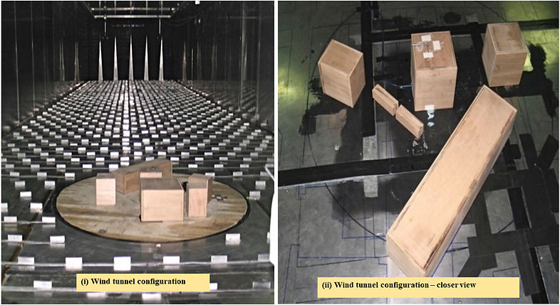
Figure II.3-5: The model installed in the wind tunnel [65].
Aristodemou et al. implemented a software called FLUIDITY which leverages the Large Eddy Simulation (LES) method to simulate complex turbulent flows. The key strength of the LES approach is that it enabled them to capture unsteady flows at high temporal and spatial resolutions [65]. Moreover, as they worked at a very large scale, they focused on tractable and accurate method. Besides, FLUIDITY can be run in parallel on multiple processors. Since the approach taken required modeling for the small scales, wind tunnel experiments were carried out to evaluate the performance of the models. A 1:200 scale tunnel model was build (Figure II.3-5) and the seven buildings were studied in isolation in the wind tunnel.
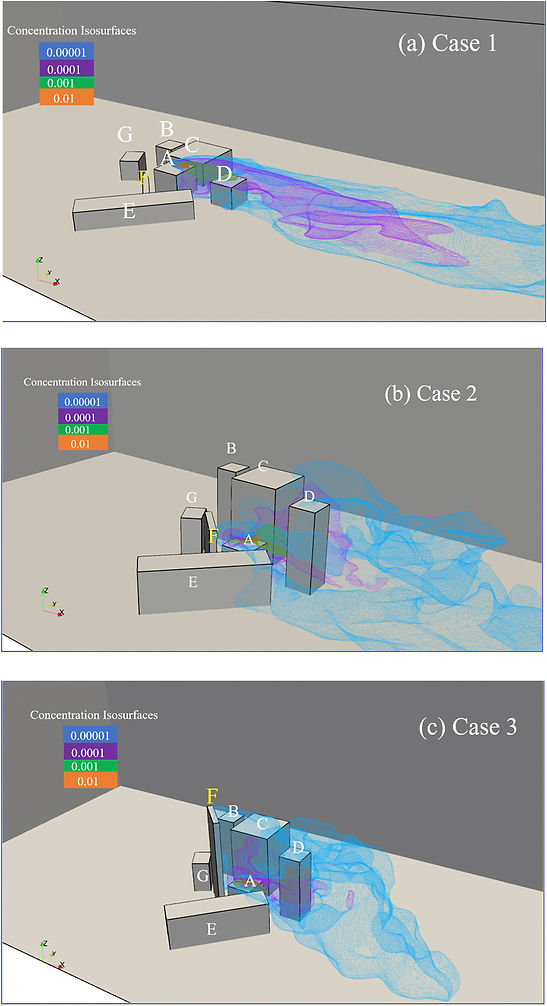
Figure II.3-6: Concentration iso-surfaces for Cases 1, 2 and 3, showing how the presence of tall buildings affects pollution dispersion within a local neighbourhood [65].
A validation study was conducted and it compared the results obtained with the LES simulation to the measurements in the wind tunnel data. The LES simulations lasted ten seconds, corresponding to the same amount of real time. The main simulated variables as functions of time were pressure, velocity, and tracer concentrations. Satisfactory correlations were observed between the observed and predicted normalised mean concentrations with a percentage of error ranging between 3% and 37% [65].
An illustration of some of the results of Aristodemou et al. experiments is given in Figure II.3-6, and demonstrates how the dispersion of air pollution is affected by tall buildings. Case 1 represents the base case. In case 2 and 3, the heights of the buildings were increased, except for building A, which was the source building for the emission of pollutants. We can see that after increasing the building heights in cases 2 and 3, rather than spreading downwind in the building area like in Case 1, the higher pollution concentrations remains within the building complex. As a matter of fact, taller buildings lead to a worsening of the pollution levels within that site. Moreover, pollutants are more easily spread into regions which were non-polluted before. They also observed that in general, the pollution-free regions are not sustained, and the vertical pollution concentrations are greatly enhanced for higher buildings. In some cases, a concentration of 300% was even detected. A complete description of the results is available in [65].
Aristodemou et al. research emphasized in a clear visual manner the importance of taking the height of building into account when designing urban environments. This was possible thanks to Computational Fluid Dynamics, which paved the way for detailed computational and physical modeling of turbulent flows. But the impact of the progress in turbulence research goes beyond the diffusion problem. The fascinating topic of energy harvesting will be addressed thereafter in the following subsection.
Energy harvesting
Energy harvesting is a process which captures small amounts of energy that would otherwise be lost to improve the efficiency of energy production. Wind is a clean and readily available renewable energy source which can reduce the dependencies on fossil fuel reserves. However, atmospheric turbulence can affect the power production of wind turbines. Turbulence vibration is generally considered undesirable, and is a phenomenon that if not properly anticipated can lead to catastrophic structural failure. However, from an energy harvesting perspective, these types of vibrations have been found to be quite valuable. Therefore, by understanding the impact of turbulence on the performance of wind turbine, we can provide the condition to efficiently capture the energy and to reduce the undesirable effects of ambient turbulence.
According to the study of Tummala et al. [74], large scale wind turbines alter the global climatic conditions and have negative effects on atmosphere. However, small scale wind turbines offer a great scope for producing valuable power which can be sufficient for domestic needs without altering the climatic conditions.
Small scale wind turbines can be classified based on different categories. There are two major types of small wind turbines based on rotation axis; the horizontal axis wind turbine (HAWT) and the vertical axis wind turbine (VAWT). The study of Pagnini et al. [75] focuses on the investigation of the power production of two small-size commercial wind turbines, with horizontal and vertical axis which characterized by the same rated power of 20 kW, installed in the Savona Harbour. The HAWT has shown to be strongly affected by gusts and large mean wind speed and direction fluctuations, however the overall energy production of that is higher than the VAWT which is less exposed to gusts and wind fluctuations.

Figure II.3-7: (Left) Horizontal Axis Wind Turbines. (Right) Vertical Axis Wind Turbines [74].
Turbulence in the approaching wind can have a significant impact on the power output of wind turbines. The goal of the study of Lubitz [73] is to investigate the effect of ambient turbulence levels on wind turbine energy production by using a small wind turbine. The studied turbine, which is a horizontal axis turbine, is located far away from obstacles in order to keep the results as general as possible and the data from disturbed sectors are not used.
In the study of Lubitz [73], the data from the turbine is divided into three categories based on turbulence intensity. Low turbulence and high turbulence intensity are classified as turbulence intensity less than 0.14 and greater than 0.18 respectively and turbulence intensity between these two values is classified as intermediate.
The measured data from Lubitz [73] shows that turbulence has a range of impacts on such systems. The interaction of the turbine with turbulent winds is complex and will vary depending on the turbine's characteristics. Also, it is found that ambient turbulent intensity impacts energy production depend on wind speeds.
Turbulence levels had a small but noticeable impact on overall power output at wind speeds between cut-in and furling which is the normal operating range. As shown in Figure II.3-8, the studied turbine has a cut-in speed of 4 m/s and begins furling at 9 m/s. Over this range of speeds, low turbulence is associated with a 2% decrease in power output. Conversely, medium and high turbulence intensity is associated with a power increase of approximately 2% in this range.
At low wind speeds, increased turbulence appears to increase the energy production of the turbine, while at high wind speeds near the turbine furling speed, low turbulence levels lead to increase the power output and elevated turbulence results in decreasing the energy production.
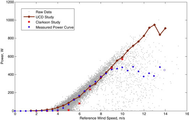
Figure II.3-8: Measured Bergey XL.1 power curve with comparisons to UCD and Clarkson studies measured [73].
Figure II.3-8 in [73] shows measured turbine power curve using a 2 Ω resistive load with comparisons to UCD and Clarkson studies using the same turbine and load. The UCD turbine is mounted on a 9 m mast on the roof of a 3 story building, on a campus surrounded by buildings and trees. It could be expected that this turbine would experience higher ambient turbulence than the Clarkson turbine or the studied turbine in [73]. Therefore, the UCD turbine has a lower cut-in wind speed at about 3 m/s than the cut-in speed observed in [73] and also in the Clarkson turbine.
It can be argued that the effect of the sites turbulence levels in large turbines is manageable. However, small turbines may be under the same or a similar condition while experiencing a wider range of ambient turbulence levels. In this regard, different approaches are proposed to address the undesirable impact of site turbulence and many technologies are developed to efficiently capture energy. For example, [76] describes a new methodology based on TRIZ principles to increase the wind speed and power output of small turbines located in urban areas. The velocity of wind in an urban location is comparatively lower than in rural or semirural locations. As shown in figure II.3-9, this study suggests the use of adjustable rooftops that could be tilted over a range of angles. This study underlines a system to reduce the passiveness time of wind turbines located in buildings. That could make urban wind turbines more agile and active resulting in higher power generation and resource utilization.
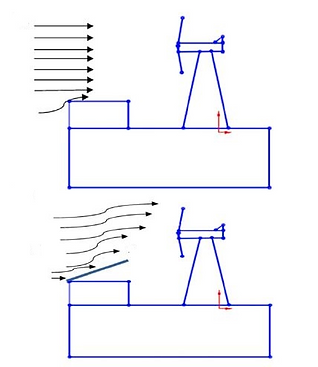
Figure II.3-9: Wind turbine and mobile sloped attachment at flat rooftop of building [76].
The impressive progress in turbulence research laid the ground for new opportunities, reflected in a wide variety of applications. This section highlighted that not only turbulence contributes to the small scale by enhancing mixing, but it also covers a much larger scale, namely the study of dispersion and energy harvesting.
Offshore wind farm [90]
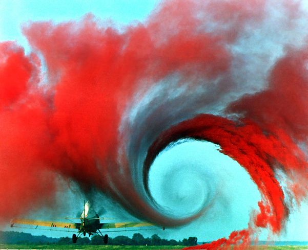
Conclusion
Turbulence research has come a long way since the first observations made by Da Vinci centuries ago. Outstanding progress have been made in computer simulations, providing a remarkable impetus to turbulence study. Direct Numerical Simulation, to give but one example, is a clear testimony of the achieved breakthrough. Yet, despite all the tools we have at our disposal today, turbulence is still a very complex phenomenon. Different points of view were adopted over time and discussed throughout this blog. To cite but a few dissensions about the nature of turbulence, the continuous versus discrete debate and the deterministic versus stochastic debate are noteworthy examples. What really marked a turning point in turbulence research was the arrival of computers, which refined numerical simulations and greatly enhanced experimentations, opening the door to a wide variety of applications. The ability to measure, sense, and control turbulence, the ability to counter it, to put up with it, and to benefit from it are direct consequences of the impressive progress in turbulence study.
Turbulence in the type vortex from an airplane wing [85]
Turbulence in the type vortex from an airplane wing [85]